The Quantification and Analysis of Second Balls in Football Part 2

In part 1, we looked into building upon Hang’s framework for extracting second ball wins from data and incorporated our own ideas such as high-order balls to create player and team statistics and heatmaps. Feel free to give it a read but if you haven’t, all you need to know for this post is the two following points.

• We have built the means to extract second balls from data.
• We look at the resulting possession following a second ball win, “the second ball possession”, which ends with a change in possession, stoppage in play, or a shot on target.

Also, both the work done in part 1 and 2, have been taken directly from my master’s thesis. I just have shortened it significantly into (hopefully) a quicker and easier read. There’s a much deeper analysis into the accuracy of every component in the model. Feel free to take a look here.

The goal of this work, is to create a methodology to give insight into the value of second ball wins, beyond just the number and location of them that occur. We do this by predicting where they occur and the attacking value they add to the second ball winning team.

On that note, let’s get into the model and analysis.

Model Overview

A model is created to estimate the attacking value from winning a second ball. It is called Expected Second Ball Value (xSBV) and is split into three components.

1. Location Prediction: where the ball is most likely to land.
2. Win Probability: probability each team will win a second ball.
3. Gain Difference: probability of scoring from a second ball win

And the model can be described below:

\[\text{xSBV} = \underbrace{P(L)}_{\text{Location Probability}} \times \underbrace{P(W \mid L, \mathbf{X})}_{\text{Win Probability}} \times \underbrace{\Delta_{i,j}P(G_H \mid W)}_{\text{Gain Difference}}\]

where:

• $L$ is the predicted location of the second ball,
• $W$ denotes the winning team (binary outcome: $W = 1$ for Team A, $W = 0$ for Team B),
• $\mathbf{X}$ represents contextual features (e.g., player positions, duel type),
• $\Delta_{i,j}P(G_H \mid W)$ is the difference in probability of a goal occurring within H transitions after a second ball win, $W$, from location $i$ to $j$.

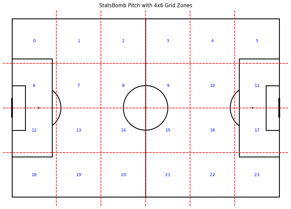
Pitch Discretization

To simplify modelling, the pitch is partitioned into a 4x6 grid. Using this grid we can get meaningful distinction between defensive, midfield, and attacking areas, as well as central and wide.

Data Set and Visualizaton

For the following analysis I use event data from the 2015/2016 English Premier League which can be found here, the StatsBomb open data github repo. It is event data and although tracking data would most likely improve the results of this work, the StatsBomb repo is all I had access too.

The distribution of second balls and where they occur can provide us with some insight about characteristics of second balls.

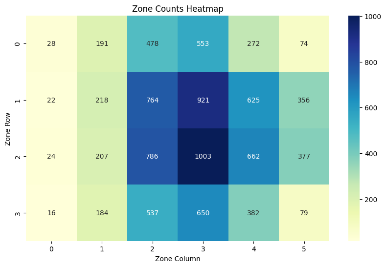
1. Second balls in the defensive third are low when compared to other thirds.
2. The middle third dominates the locations of second balls.
3. Second balls are less likely to occur in wide areas.

Features

Thirteen features were created to capture the spatial and contextual dynamics of second balls. These components were taken from the event data

Feature Name	Description
pass_start_x, pass_start_y	x and y coordinates of the starting location of the initial long ball.
pass_end_x, pass_end_y	x and y coordinates of the ending location of the initial long ball.
pass_distance	Length of the initial long ball.
pass_angle	Angle in radians of the initial long ball to the goal.
dx, dy	Change in x and y coordinates of the start and end location of the initial long ball.
dist_to_centre	Distance of the end location of the initial long ball to the centre of the field.
is_defensive, is_midfield, is_attacking	Boolean flags to indicate what third of the field the end location of the long ball occurs in.
is_contested	Boolean flag to indicate if the initial long ball is met with a duel, e.g. ADBA, ADAA, ADAB, or ADBB (see previous post).
second_x, second_y	x and y coordinates of the second ball location.
has_transition	Boolean flag to indicate if there is a transition period in the second ball win or not.

Location Prediction

Objective: Predict the zonal location of where a second ball occurs given a list of features.

Model Formulation

Let $p_0$ be the initial duel location and $X_{context}$ be a list of features. The second ball location, $L$, is modelled as a stochastic outcome:

\[P(L_z \mid p_0, X_{context})\]

where $L_z$ is the corresponding zone that location $L$ belongs to and

\[\begin{aligned} X_{context} = \{&\text{pass_start_x, pass_start_y, pass_distance, pass_angle,} \\ &\text{dx, dy, dist_to_centre, is_defensive, is_midfield,} \\ &\text{is_attacking, is_contested}\} \end{aligned}\]

Modelling Techniques

The location prediction task is a multi-class classification problem (Singh, 2024), where the goal is to predict the pitch zone where the ball is most likely to land after a contested aerial action or clearance. Each instance is assigned a class label based on the observed ball destination. To model this, Extreme Gradient Boosting (XGBoost), a powerful gradient-boosted decision tree algorithm (Chen & Guestrin, 2016) is used. Due to the multi-class nature of the task, the model is trained using softmax objective with log-loss as the optimization criterion. Model performance is evaluated using top-k accuracy metrics (Ghosh et al., 2025), specifically top-1 and top-3, to assess how often the true location falls within the top predicted zones.

Second Ball Winning Team Prediction

Objective: Estimate the probability that a given team wins the second ball at location L.

Model Formulation

A binary classifier predicts:

\[P(W = Team_A \mid L, X_{context})\]

where $W$ denotes a second ball win and

\[\begin{aligned} X_{context} = \{&\text{pass_start_x, pass_start_y, pass_distance, pass_angle,} \\ &\text{dist_to_centre, is_defensive, is_midfield, is_attacking,} \\ &\text{is_contested, second_x, second_y, has_transition}\} \end{aligned}\]

Modelling Techniques

The task of predicting which team will win a second ball is formulated as a binary classification problem (Karabiber, n.d), where the model must determine whether the team initiating the long ball or the opposing team will gain possession following the contest. Three machine learning models are used to address this problem: XGBoost, Random Forest, and Logistic Regression. Random Forest is an ensemble method that combines multiple decision trees to reach a single result, offering resistance to overfitting, especially when the feature space is large and noisy (Biau & Scornet, 2016). Logistic Regression provides a simple and interpretable model, relying on a linear combination of input features passed through a sigmoid function to estimate the probability of each class (GeeksforGeeks, 2016). Comparing these models allows for an evaluation of accuracy between different models.

Gain

To quantify the probability that a goal occurs in the possession after a second ball win, a Markov chain model called gain is proposed. This approach is similar to (Rudd, 2011), (Singh, 2018), and (Fernandez et al., 2019), but adjusted to my problem, which captures both immediate and transitional danger of second balls. This is basically my attempt at implementing expected threat.

Markov Chains for Possession Transitions

A Markov chain is a probabilistic model that represents a system transitioning between discrete states, where the probability of moving to the next state depends only on the current state and not the sequence of events that precedes it (Sekhon & Bloom, 2020). The assumption that the next state depends only on the current state, known as the Markov property, is a simplification that enables efficient modelling of second ball possessions. In reality, past actions may influence future outcomes, but this assumption is reasonable in a football context. For instance, there are many ways a team might advance the ball into the attacking third. However, once the ball is in the attacking third, the likelihood of scoring or losing possession is mainly determined by the current position and state of play, rather than the actions that led there. Absorbing states are such that once transitioned into, they cannot be left. In my context, there are two absorbing states: a goal and the end-of-possession. Transitions represent the movement of the ball between states. A transition matrix is constructed using observed transitions from the data, and convergence is used to estimate the long-term trends of the absorbing states. Below is the transition matrix.

\[P = \begin{bmatrix} p_{z_0, z_0} & p_{z_0, z_1} & \cdots & p_{z_0, z_{23}} & p_{z_0, z_g} & p_{z_0, z_{eop}} \\ p_{z_1, z_0} & p_{z_1, z_1} & \cdots & p_{z_1, z_{23}} & p_{z_1, z_g} & p_{z_1, z_{eop}} \\ \vdots & \vdots & \ddots & \vdots & \vdots & \vdots \\ p_{z_{23}, z_0} & p_{z_{23}, z_1} & \cdots & p_{z_{23}, z_{23}} & p_{z_{23}, z_g} & p_{z_{23}, z_{eop}} \\ 0 & 0 & \cdots & 0 & 1 & 0 \\ 0 & 0 & \cdots & 0 & 0 & 1 \end{bmatrix}\]

The Markov chain framework is well-suited to this problem due to its interpretability, simplicity, and ability to capture the stochastic nature of ball progression in football. Formally, the possession evolution is modelled as a Markov process where:

• Transient States: The 24 grid zones ${z_1, \ldots, z_{24}}$
• Absorbing States: Goal and End-of-Possession ${z_g, z_{eop}}$
• Transitions: Probabilities $P(z_j \mid z_i, W)$ are estimated from historical data, conditioned on the winning team $W$.

Convergence of the Transition Matrix

Each multiplication of the transition matrix $P$ by itself represents an additional step in the possession sequence. Specifically, $P^n$ describes the probabilities of reaching any given state after $n$ transitions (Permana et al., 2018). For second ball possessions, the probability of a possession eventually reaching one of the absorbing states is of interest. By repeatedly multiplying the matrix by itself, these probabilities change and eventually stabilize. This process is known as convergence. In practice, the matrix is repeatedly multiplied by itself until there is a small enough state difference between iterations. The difference threshold value is arbitrarily chosen, and in this work 0.025 is used. Convergence allows for the long-term distribution of second ball possessions to be determined.

Model Formulation

Horizon-Limited Markov Chain

Let $\mathbf{P_t} \in \mathbb{R}^{24 \times 24}$ denote the probability transition matrix between transient states, and let $\mathbf{P_g} \in \mathbb{R}^{24 \times 1}$ denote the column vector of transition probabilities from each transient state into the absorbing state “Goal”. For a fixed horizon $H$, the cumulative probability of absorption in the Goal state within $H$ steps, or gain, is

\[P(G_H) = \left(\sum_{h=1}^{H} P_t^h\right) P_g \tag{3.6}\]

Where:

• $\mathbf{P_t^h}$ gives the distribution of transient states after exactly $h$ steps.
• multiplying by $\mathbf{P_g}$ projects these distributions onto the probability of transitioning to Goal.
• summing over $h$ accounts for scoring at any step up to horizon $H$.

Gain Difference

The gain difference $\Delta_{i,j}P(G_H)$ is defined as the difference between the cumulative probability of scoring a goal within $H$ steps of zones:

\[\Delta_{i,j}P(G_H) = P(G_H)[j] - P(G_H)[i] \tag{3.7}\]

where $P(G_H)[n]$ is the $n$th element of $P(G_H)$, i.e., the probability of scoring within $H$ steps when starting in zone $z_n$.

Expected Gain

Let $\mathbf{P_{first}} \in \mathbb{R}^{24 \times 24}$ be the empirical distribution of the first successful team action destination conditioned on the start zone. Multiplying the first-action matrix with the expected scoring value and then subtracting the probability of scoring in $H$ steps from starting zone $z_i$ gives the expected gain for the first action following a second ball win.

\[xP(G_H, z_i) = P_{first} P(G_H) - P(G_H)[i] \tag{3.8}\]

Comparing expected gain to the actual gain players receive from second ball wins provides insight into which players underperform or overperform relative to expectations. Due to time constraints, I didn’t implement this in my work, but is a natural extension.

Component Performance

After training the components using the above methodology, we evaluate the accuracy and performance of each.

Location Prediction

Rather than relying solely on the top-1 predicted location for second balls, this work adopts a top-3 prediction strategy. In the context of football, the landing zone of a second ball is uncertain due to seemingly chaotic nature. By considering the three most probable zones, a more realistic representation of how the model is thinking and where it is predicting the second balls to land is captured. Additionally, top-3 evaluation reduces the harshness of strict classification accuracy and better reflects the model’s value in practical settings where anticipating a region, rather than a single zone, can inform decision-making.

Model	Top-1 Accuracy	Top-3 Accuracy	Log Loss
XGBoost	0.2382	0.6022	2.6712
Naive Baseline	0.1063	0.2849	-

The location prediction component achieved a 23.8% top-1 and 60.2% top-3 accuracy. While these numbers indicate low prediction accuracy, they are notable given the complexity and novelty of the task. A naive baseline approach, simply predicting the most common zones, only has an accuracy of 10.6% top-1 and 28.5% top-3 accuracy. Significantly outperforming the naive baseline suggests the model is not random and has some ability to learn spatial patterns. Despite room for improvement, these results mark an important result in quantifying and modelling second ball outcomes in football.

Winning Team Prediction

To evaluate the performance of the team winning prediction component, three core metrics are reported: accuracy, log loss, and the area under the receiver operating characteristic curve (AUC-ROC). AUC-ROC offers a more nuanced evaluation by measuring the model’s ability to distinguish between positive and negative classes (Naidu et al., 2023). An AUC-ROC score of 0.5 indicates random performance, whereas a score closer to 1.0 reflects strong discriminatory power. Log loss and accuracy are once again included to further help analyze the model performance.

Model	Accuracy	AUC-ROC Score	Log Loss
Logistic Regression	0.704	0.761	0.584
Random Forest	0.718	0.790	0.554
XGBoost	0.722	0.799	0.548
Naive Baseline	0.585	0.5	-

In the table above, it is shown that although all three models perform similarly, XGBoost is marginally the best. It is more important that the naive baseline of always predicting team B as the winner of the second ball is outperformed. With a slightly imbalanced dataset, predicting team B every time results in an accuracy of 0.585, significantly lower than the best accuracy of 0.722. Another important note is the AUC-ROC scores of the final models. All models are upwards of 0.75, with the best being 0.799. These scores provide a good indication that the models are reliable and meaningfully confident at discerning between winning and losing outcomes

Gain

Visualizing Convergence

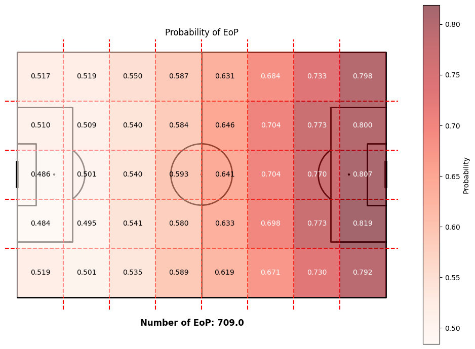
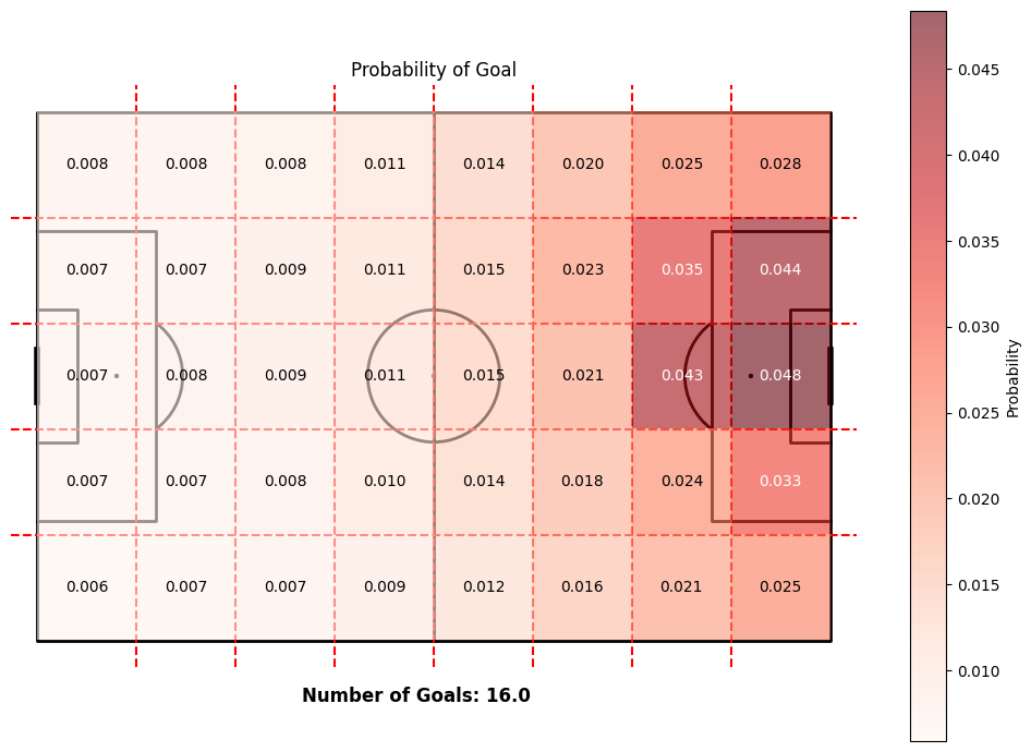
To get an intuition for how the long-term distribution of second ball possessions emerge, the heat maps of the absorbing states can be observed. The figures below shows the probability of the possession ending after 20 transitions. There is a clear pattern that the closer the team in possession gets to the opponent’s goal, the more likely the possession will end. Again, this is trivial, but now we have evidence to back up the claim. The figures also show the probability of a goal after 20 transitions. Again, there is a clear pattern that the closer the team in possession gets to the opponent’s goal, the more likely they are to score.

Zone Valuation

Visualizing the gain per zone can provide insight into how areas of the pitch are valued. Unless otherwise stated, the analysis will be conducted using H = 5 (goal of occurring in next 5 transitions).

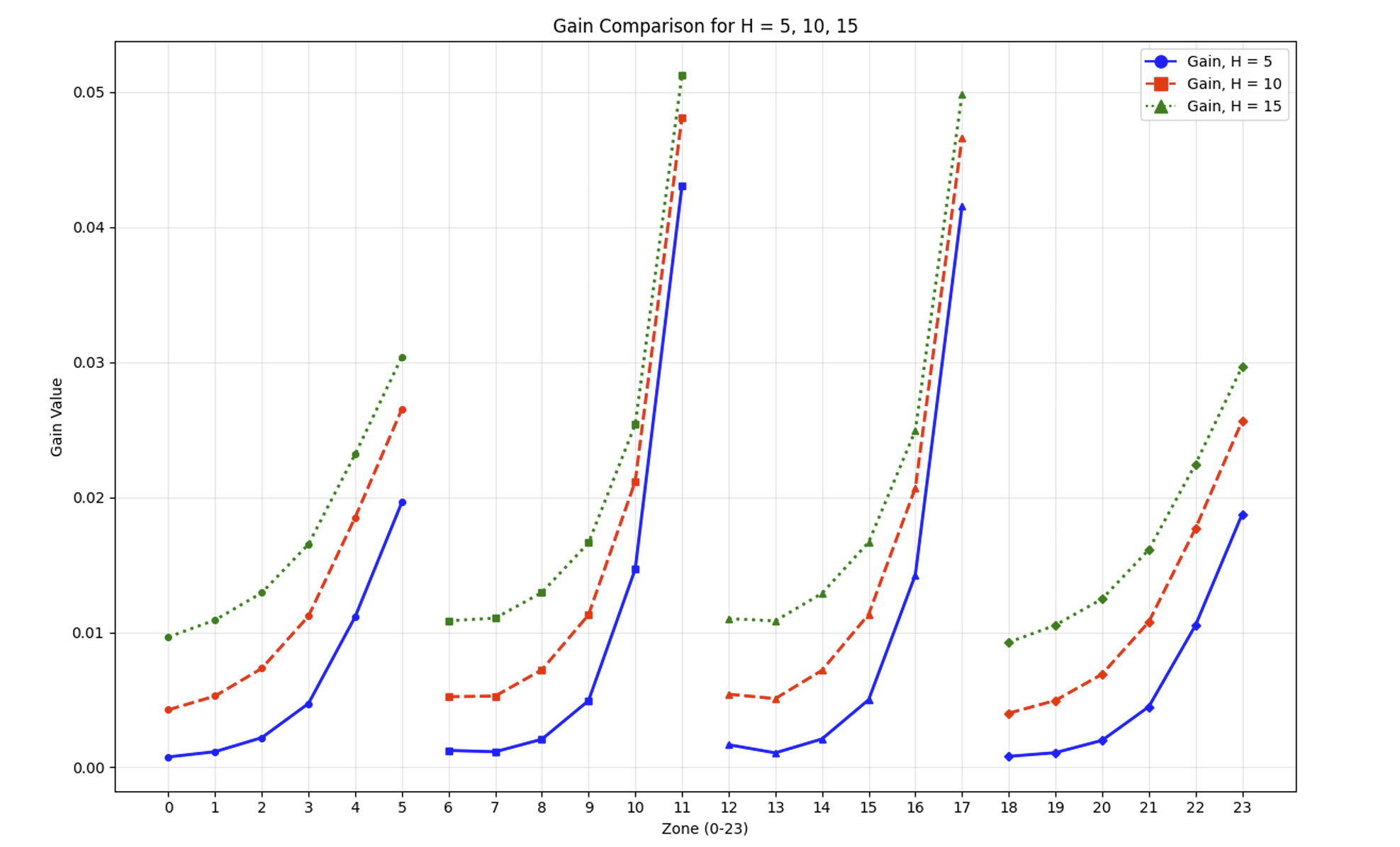
As expected, the cumulative probability that a goal occurs in the next H actions increases as H increases. Similarly to the convergence probabilities, we see that for H = 5, 10, 15, the closer and narrower a player is to the opponent’s goal the more likely a goal will occur.

Bootstrapping

To quantify the uncertainty in the gain component, the bootstrap, a resampling technique, is used. Bootstrapping uses an observed sample to construct a statistic’s sampling distribution (Beasley & Rodgers, 2012). The observed median from the original sample of N scores is calculated. An empirical sampling distribution is created by repeatedly drawing N random samples with replacement from the dataset of second ball possessions. Drawing N random samples is considered one bootstrap sample. This process is repeated B = 1000 times. The bootstrap distribution is formed by calculating the median for each bootstrap sample.

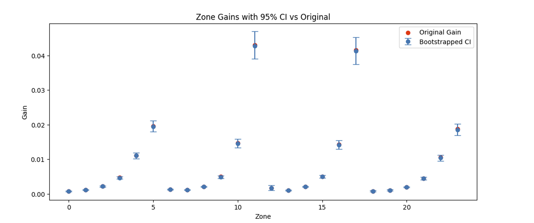
From the above figure, it is clear that the original gain scores are very similar to the bootstrapped medians. Confidence intervals are minimal from defensive zones and appear to grow towards attacking zones. Having more uncertainty in attacking zones is not surprising since there are fewer samples. However, the attacking zones’ confidence intervals are not large, which gives evidence that the bootstrapped gain distribution is valid.

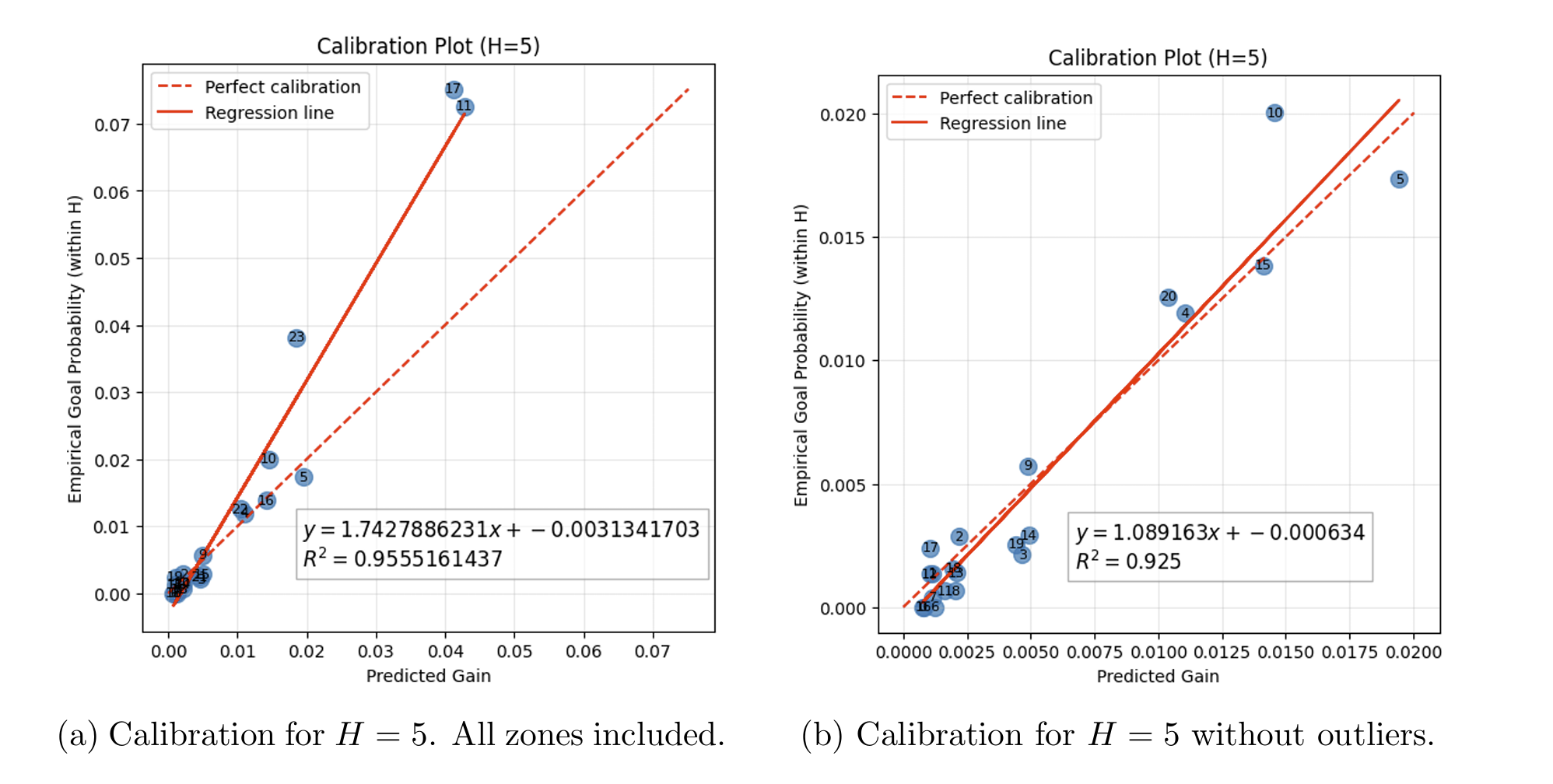
Calibration

The calibration of the gain was assessed by plotting empirical probabilities against predicted probabilities. The initial regression slope of approximately 1.7 indicates calibration issues compared to the perfect calibration slope of 1. Excluding zones 11, 17, and 23 decreases the slope to 1.089, which is very strong. The outliers have low empirical counts since they are attacking zones, suggesting the empirical probability does not reflect the underlying gain distribution. However, for the majority of zones, the Markov chain framework produces well-calibrated estimates.

Player Analysis

Now for the main result of this thesis, the xSBV for players. The table below shows the average xSBV for players with more than thirty-eight second ball wins. The cumulative xSBV is also shown along with the average and cumulative gain difference. The total number of second balls won from each player is also listed. It is noted that second ball wins that are won and transitioned into the same zone are not counted since the gain would equal zero. The zones that are not counted are a significant limitation of the xSBV model and are discussed in the limitations section towards the end.

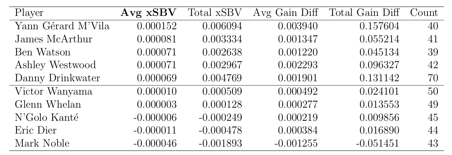
Yann Gerard M’Vila leads the list with the highest average xSBV (0.000152), supported by a relatively strong total gain differential (0.1576) across 40 events. The others in the top 5 have similar average xSBV scores, but considerably lower then M’vila. Therefore, in terms of creating value from second ball wins, it is concluded that Yann M’vila is the best. As a midfielder from Sunderland who would not widely be regarded as a “top” midfielder, it is exciting that the metric shows him as the best in the Premier League with respect to improving a team’s chances of scoring from second ball wins. Looking back at the Premier League table, we notice that Sunderland finished in 17th place, avoiding relegation by one spot.

At the opposite end, Victor Wanyama and Glenn Whelan post near-zero averages, and N’Golo Kante, Eric Dier, and Mark Noble register negative values. However, it is crucial to note that these metrics only capture the probability of goals and do not reflect defensive value. Many of the lower-ranked players are defensive midfielders whose primary role is to disrupt opposition play and secure possession with safe passes. Without the value of the opponent winning the ball, we cannot fully capture the importance of these players. However, we can use average gain and cumulative gain and cumulative gain to get a better idea of their importance.

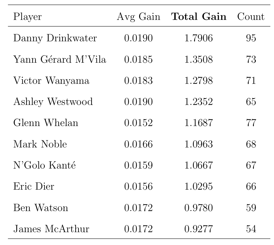
Even without accounting for defensive contribution, the table above shows the importance of defensive midfielders. Victor Wanyama and Glenn Whelan both have entered the top 5 comparatively, while the rest have similar scores. So by using part of the full metric, the zonal value of player’s second ball wins can be seen.

Team Analysis

Now, the xSBV scores per team can be analyzed. Again, the teams are ranked in order of highest xSBV to lowest.

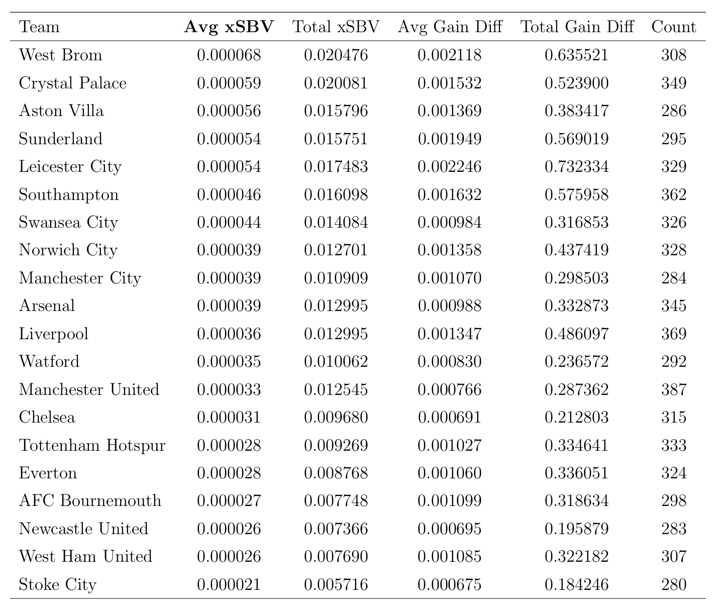
The above figure reveals some interesting results. Originally, it was thought that lower table teams would have worse xSBV, but that is not necessarily the case. A more reasonable explanation would be that high xSBV would be associated with teams with a direct, long-ball play style. So it makes sense that worse teams already focus on quick attacks following second ball wins. However, not all lower table teams have high xSBV. For example, Newcastle, the team that was closest to avoiding relegation, had the third worst xSBV score. The lower score indicates that Newcastle could have benefited from improvements in attacking play following second ball wins. Cases like Newcastle are exactly who this metric is geared toward. There is a possibility that if Newcastle had worked to improve their xSBV, they could have avoided relegation.

To provide coaches and players with tactical guidance for winning second balls, heat maps are presented, which show trends of where second balls are likely to land. Although the location prediction component does not predict zones with high accuracy, it does seem to understand the spatial relationships of second ball win locations. As component performance is improved, a similar location distribution is expected, but with higher prediction accuracy.

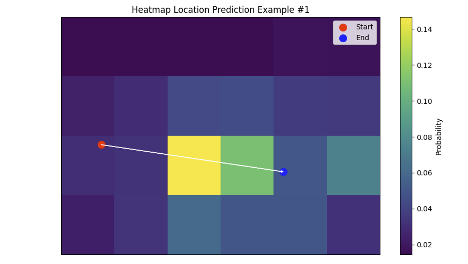
However, from the above figure, it can be shown that a long ball from zone 12 to 16 is most likely to fall into zones 13 and 14. It is also noted that zone 17 has the next highest probability. Therefore, a tactic could be to target zone 16 from goal kicks with many players in zones 13 and 14, with a few players running in behind to zone 17 for flick-on headers. This is one example, but by looking at team-specific visuals of where past success occurred, coaches can use the ideas from the location prediction component to create new tactics for their team.

Limitations and Future Work

It goes without saying as my first real attempt at football analytics and modelling, this novel work has no shortcoming of limitations. With many of these limitations however, come new questions and future work that can be built upon.

The biggest limitation belongs to the data used. Without access to tracking data, event data was used, almost certaintly missing out on valuable predictive information that would help strengthen the model. Knowing the locations of players should help improve predictions on all fronts, from where the second ball occurs to which team is most likely to win it. A natural extension would be to reproduce these components with tracking data to see how accuracy improves.

Also, the methodology is inherently flawed as manual annotation of games were used to identify second ball scenarios. Certain edge cases are very likely to have been missed, meaning there still is no way to extract all second balls with 100% accuracy. That being said this method still provides a way to highly increase the speed at which many second balls can be extracted, compared to manually having to annotate games by hand.

Set pieces are also not included in the analysis. This was due to scope of research and the difference in nature of open play and set pieces. I believe results most likely would be different and so including set pieces in the same analysis could have taken away from the results. A simple extension to investigate second balls from set pieces would be a natural and interesting pathway forward.

Also, only second ball wins were analyzed. In reality, ignoring second balls where possession was not established contributes to a lower number of second balls per game, and potential game dynamics that are left unexplored. For example, second balls where possession is never immediately established maybe is where real oppurtunity lies for teams to improve on their number of second ball wins.

For the gain component, the model assigns scores by using the difference in probability of scoring a goal within the near future from two different zones. The problem is that if the second ball winner gets the ball and transitions it to the same zone, the resulting difference in gain would equal zero. In reality, the difference should not be zero since winning the second ball itself provides value for your team, regardless of where you transition it to. Continuing with this, the defensive value of winning a second ball is massive as it is stopping your opponent from making transitions that improve their teams chances of scoring, which is not inlcluded in gain since its purely a goal scoring metric. Improving or creating a new way to understand the value second ball wins add to the defense as well as the attack is a natural extension.

Last, the values from the xSBV model are hard to interpret. Since the values from each component are very small due to accuracy of components, the xSBV becomes very small. In retrospect, the need to combine all components into a single output was probably not necessary as each part by itself can be useful in its own right. The idea of having a single metric with a fancy name definetly sucked me in. However, the metric can still be used as comparing players within the metric still works as the scores are relative. Thus, we still established rankings of players and teams.

This is by no means as an exhaustive list, and there’s many more in my actual thesis. I wanted to get my favorite limitations and ideas for future work in this post as I think they may have the most value in providing others with ideas while understanding where my work falls short.

Conclusions

If you have made it this far, I would like to say thanks! This thesis marked a big chapter in my life and I am glad that I was able to shrink it down into a (somewhat) more tolerable verision. At the beginning I had two simple goals. The first to follow my passions and create a project in football analytics. The second was to come up with an idea that was relatively (if at all) unresearched and see what I could come up with. Although, it is nothing ground breaking, I am quite proud to have seen it through from start to finish. Along with that I think there are some cool ideas and insights sprinkled throughout and I have definitely learned a lot and will be a better researcher and football analyst beacuse of it. I look forward to continuing improving my analytics skills and hopefully create cooler and better things in the future. As always any comments or feedback would be appreciated so feel free to reach out on Twitter or email.

Jack Sears